Discrete spatial samples
Explicit XYZ samples with optional color, intensity, normal, class, uncertainty, or time. A point set does not automatically define a continuous surface or view-dependent appearance.
 Pajama StudioSpatial Rendering Field Guide
Technical field guide · 3DGS · 4DGS · Dynamic view synthesis
A systems-level guide centered on 3D and 4D Gaussian Splatting: how Gaussians are learned, activated, projected, composited, moved through time, encoded, delivered, and validated. Point clouds and NeRF provide the comparison needed to understand what is genuinely different.
First principles
Explicit XYZ samples with optional color, intensity, normal, class, uncertainty, or time. A point set does not automatically define a continuous surface or view-dependent appearance.
A network or accelerated field answers density and color queries at a position and viewing direction. Pixels come from samples integrated along camera rays.
A set of anisotropic Gaussians with position, covariance, opacity, and appearance. Each Gaussian projects to a screen-space ellipse and contributes through alpha compositing.
Dynamic methods add time, motion, deformation, or per-frame state. Their temporal models and file schemas are method-specific rather than one universal 4D format.
| Question | Point cloud | NeRF | 3DGS | Dynamic GS |
|---|---|---|---|---|
| Core representation | Point samples | Continuous radiance/density function | Explicit Gaussian set | Gaussians plus a time model |
| Pixel generation | Point or surfel rasterization | Ray sampling and volume integration | Project, order/bin, splat, composite | Evaluate time state, then splat |
| Geometry | Positions, no connectivity | Implicit density | Centers and covariance, no mesh topology | Time-varying centers, shapes, or features |
| View-dependent appearance | Usually absent | Native viewing-direction input | Often spherical harmonics | Method-dependent |
| Typical cost | Bandwidth, LOD, holes | Field evaluations per ray | Ordering, overdraw, memory | Those costs plus temporal evaluation |
Interactive representation lab
Orbit a real GPU camera, zoom, change time, and switch the rendering contract. Point Cloud, 3DGS, and STG reuse the same published STG-Lite asset; the NeRF tab is an explicitly labelled procedural neural-field analogue because this site does not ship a trained NeRF checkpoint.
The camera projects the asset’s actual XYZ centers as circular point primitives. A depth buffer resolves visibility; no Gaussian scale, rotation, opacity, or temporal motion is evaluated.
Raw observations include optics, exposure, sensor noise, timestamps, and coordinate conventions.
SfM, SLAM, or calibration recovers cameras and often a sparse structure.
Choose the scene function and parameters to optimize or reconstruct.
A research checkpoint and deployable asset are often different formats.
Camera transforms, visibility, shading, and compositing produce pixels.
Training ↔ rendering connection
At training time, the rendered pixel is differentiable with respect to network or feature-grid parameters.
At training time, differentiable splatting updates position, covariance, opacity, and appearance; adaptive density control changes the primitive set.
Both methods compare rendered pixels with captured pixels and differentiate through the renderer. Their central difference is the optimized scene representation and the rendering operator—not the supervision signal.

The original project diagram connects posed input images to field optimization and novel-view rendering. Image © the paper authors; shown for technical commentary.

SfM points seed Gaussians; projection and a differentiable tile rasterizer close the image-loss loop while density control changes the primitive set. Cropped from the original paper.
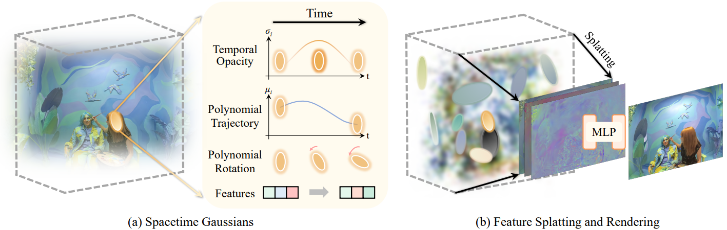
Temporal opacity, polynomial motion and rotation, and time-dependent features are evaluated before feature splatting and image decoding. Image © the paper authors.
The most important distinction
How bytes are arranged, compressed, and chunked: PLY, LAS, E57, SPZ, SOG, or GLB. This answers how data is stored and transported.
The fields, types, order, and counts: PLY properties such as x/y/z, or Gaussian scale, rotation, opacity, and SH coefficients.
What values mean: linear or log scale, alpha or opacity logit, quaternion order, SH basis, units, axes, and camera convention.
How attributes become pixels: GL_POINTS, oriented surfels, ray integration, or covariance projection, sorting, and alpha compositing.
Whole-file loading versus chunks, spatial trees, temporal segments, and LOD; whether decoding yields GPU-ready data.
Interactive contract inspector
.ply extension“PLY is the Gaussian Splatting format.” A better answer is: “PLY is an extensible container commonly used for research interchange. A specific property schema, activation convention, and rendering contract make one PLY a 3DGS or STG asset.”
Explicit sensor samples
The minimum record is (x,y,z). Real datasets may also carry RGB, LiDAR intensity, return number, classification, normal, timestamp, sensor origin, or uncertainty. Points have no edges or faces by default, so a point cloud is not a mesh.
Sources include LiDAR, structured light, stereo or depth fusion, sparse/dense photogrammetry, and simulation. Whether a point represents a surface, free-space boundary, or noisy return depends on acquisition.
Good for measurement, labeling, registration, spatial queries, and large-area mapping.
New viewpoints may reveal holes. Larger points hide gaps but blur boundaries and increase overdraw.
Geospatial coordinates can jitter in float32. Use local origins, quantization, hierarchical tiles, and range requests.
Implicit continuous field
Fθ(x, d) → (σ, c)A spatial position x and viewing direction d enter the field; it returns volume density σ and view-dependent color c. Original NeRF learns this function from images with known camera poses.
r(t) = o + t·dGenerate a ray from the camera through each pixel.
αᵢ = 1 − exp(−σᵢδᵢ)Convert density over an interval into absorption probability.
Tᵢ = ∏ⱼ<ᵢ (1 − αⱼ)Energy reaching the sample without earlier absorption.
C = Σᵢ Tᵢ αᵢ cᵢIntegrate color from near to far along the ray.
Original NeRF performs many MLP queries per pixel. A product called a “NeRF viewer” may instead render a hash grid, sparse voxel grid, tensor factorization, or baked representation. The family name does not define runtime.
There is no universal deployment file. Framework-specific weights, config, and camera metadata are common. Exporting to a mesh or baked grid changes the rendering contract.
NeRF gets continuity from a queryable field and spends work on samples along rays. 3DGS gets continuous footprints from explicit Gaussians and spends work on visible primitives, ordering, rasterization, and overdraw.
Core topic · static radiance fields
3DGS is simultaneously an optimized scene representation, a differentiable training system, and a visibility-aware rasterizer. Keeping those three layers separate makes the method much easier to reason about and implement.
G(x)=exp(−½(x−μ)ᵀΣ⁻¹(x−μ))Covariance factorizationΣ = R(q) · diag(exp(s)²) · R(q)ᵀExplicit means, rotations, scales, opacity parameters, and directional appearance. There is no triangle connectivity and no density MLP to query at runtime.
Render posed training views, compare them with captured pixels, backpropagate into attributes, and adapt representation capacity through densification and pruning.
Activate attributes, transform and cull, project covariance, bin/order footprints, evaluate covered pixels, and alpha composite.
| Concept | Typical stored parameter | Runtime interpretation | If interpreted incorrectly |
|---|---|---|---|
| Scale | Three unconstrained log-scale values | s = exp(ŝ), then build Σ = R diag(s²) Rᵀ | Negative or wildly mis-sized footprints |
| Rotation | Four quaternion components | Normalize, apply the contract's component order, convert to R | Rotated, mirrored, or unstable ellipses |
| Opacity | An unconstrained logit | α₀ = sigmoid(o) | Everything disappears or saturates |
| Appearance | DC + higher-order SH coefficients | Evaluate basis using the camera-to-Gaussian direction, then apply the color convention | Wrong color, SH banding, or reversed view dependence |
| Position | XYZ in the training scene frame | Apply world/view/projection conventions and scene normalization | Misalignment, flips, or clipping |
Σ₂D ≈ J · W · Σ₃D · Wᵀ · JᵀThe view transform W and local perspective Jacobian J turn an ellipsoid into a screen-space ellipse. Implementations add numerical safeguards and footprint bounds.
αᵢ(p) = α₀ᵢ · exp(−½ Δpᵀ Σ₂Dᵢ⁻¹ Δp)A pixel receives a weighted contribution based on its offset from the projected mean. The practical rasterizer evaluates only the bounded screen footprint.
C(p)=Σᵢ Tᵢ αᵢ cᵢ(d), Tᵢ=∏ⱼ<ᵢ(1−αⱼ)Color depends on both the view-conditioned appearance and the depth order. Tile sorting is an efficient visibility approximation, not ordinary z-buffer replacement.
Recover intrinsics, poses, and a sparse point cloud with calibration or SfM.
Seed means from sparse points and initialize scale, rotation, opacity, and SH.
Select a training camera and differentiably splat the current primitives.
Compare predicted and captured pixels; the original method combines L1 and D-SSIM terms.
Update attributes, clone small high-gradient primitives, split large ones, and prune weak contributors.
Preserve the training contract or convert, quantize, and package for the target runtime.
Apply exp, sigmoid, quaternion normalization, and appearance conventions.
Reject behind-camera, off-frustum, or negligible projected footprints.
Create the 2D conic and a conservative screen-space bounding region.
Associate each Gaussian with the tiles touched by its footprint.
Sort/bin by tile and depth, then evaluate conics for covered pixels.
Accumulate transmittance-weighted color and stop when little light remains.
Interactive alpha-order lab
Depth order changes the output when translucent layers differ. Opaque points can use z-buffer replacement; alpha splats need ordering, an order-independent approximation, or explicit assumptions.
Blur, reflections, exposure shifts, sparse coverage, or bad poses can be absorbed into unstable geometry and appearance.
Tiny footprints, aggressive culling, missing antialiasing, and LOD changes can shimmer during motion.
Large overlapping splats stress approximate order and fragment bandwidth; one giant splat can touch many tiles and pixels.
Spherical harmonics encode captured directional appearance. They do not recover editable materials, lights, or physically correct unseen geometry.
The original method jointly optimizes position, anisotropic covariance, opacity, and directional appearance against posed images. The projected ellipse, translucent overlap, visibility ordering, and adaptive density control are the method—not decoration around a point cloud.
Core topic · dynamic radiance fields
In this guide, 4D means 3D space plus time. It does not imply one literal 4×4 covariance, one training algorithm, or one file format. The decisive question is: what persists, and what function produces the Gaussian set at time t?
Each Gaussian carries temporal opacity, parametric motion/rotation, and time-dependent features. Evaluate those functions at t, remove inactive primitives, then use a Gaussian splat pipeline.
| Family / example | Where time lives | What persists | Strength | Cost / limitation |
|---|---|---|---|---|
| Frame sequence / flipbook | File or buffer index | Nothing is required to correspond | Simple playback and exact per-frame capacity | Repeated storage; weak identity and interpolation |
| Persistent trajectories Dynamic 3D Gaussians | Per-frame positions and rotations with local-rigidity regularization | Color, opacity, and size remain persistent in the published method | Dense tracking and editable trajectories emerge with reconstruction | Needs suitable multi-view temporal capture and motion constraints |
| Canonical + deformation 4D-GS / Deformable 3DGS | A time-conditioned encoder/field predicts offsets from canonical Gaussians | Canonical primitive identity | Compact continuous-time deformation and familiar static splat backend | Field evaluation adds runtime work; topology/emergence remain difficult |
| Per-Gaussian spacetime STG | Temporal opacity, motion, rotation, and optional features per primitive | A primitive exists over learned temporal support | Temporal culling and local motion are explicit | Richer records and a method-specific feature/color decoder |
Acquire timestamped video, ideally with synchronized cameras and controlled exposure.
Estimate intrinsics, extrinsics, distortion, and the temporal alignment used by supervision.
Initialize frames, persistent tracks, a canonical set + field, or spacetime primitives.
Evaluate the time model and differentiably render the matching camera/timestamp.
Use image loss plus method-specific motion, smoothness, rigidity, or temporal constraints.
Test held-out views and times; inspect flicker, motion consistency, occlusion, and seek behavior.
Map playback time into the model's normalized or captured time domain.
Read a frame or compute deformation, trajectory, rotation, opacity, and features.
Drop inactive or negligible primitives before projection when the contract permits.
Produce current means, covariance factors, opacity, and appearance.
Motion invalidates a static camera-depth order; update visibility structures.
Project the current Gaussian set and run the static image-formation backend.
dt = t − μᵗ
μ(t)=μ₀ + b₁dt + b₂dt² + b₃dt³
w(t)=exp(−(dt / exp(sᵗ))²)
α(t)=sigmoid(o) · w(t)
q(t)=normalize(q₀ + dt·ω)
The selected lightweight checkpoint stores direct RGB rather than the full paper's splatted-feature decoder. These equations are implementation-specific and must not be generalized to every method called “4DGS.”
The binary little-endian PLY stores exactly 32 float32 values per vertex: base XYZ, temporal center/scale, unused normal slots, nine cubic-motion coefficients, direct RGB, opacity logit, log scale, base quaternion, and quaternion-rate coefficients.
The parser validates names, order, type, and record width. A different 128-byte record is not automatically compatible.
Unsynchronized cameras observe different object states. A representation may blur or duplicate motion to satisfy contradictory supervision.
Polynomial trajectories suit local motion segments; deformation fields offer different capacity and regularization. Both encode assumptions.
Temporal opacity can model limited support, but persistent identity becomes ambiguous when surfaces reveal, collide, tear, or leave the capture volume.
Use held-out camera/time pairs, temporal metrics or optical consistency, calibrated source comparison, and explicit playback/seek performance.
Source, interchange, delivery
| Format | Primary content | Useful property | Do not assume |
|---|---|---|---|
| PLY | Generic properties; points, meshes, research GS schemas | Simple, extensible, ASCII/binary | PLY defines no GS activation, SH, coordinates, or time semantics |
| PCD | Point Cloud Library fields | Robotics and computer vision | It is not a radiance-field runtime |
| LAS / LAZ / COPC | LiDAR, classes, returns, CRS | Geospatial ecosystem and hierarchical access | The goal is measurement/query, not novel-view synthesis |
| E57 | Multiple scans, metadata, optional imagery | Cross-scanner exchange | Runtime usually still converts and chunks it |
| NeRF checkpoint | Network/grid weights plus configuration | Preserves one training representation | No universal cross-framework “.nerf” contract exists |
| 3DGS training PLY | Mean, scale, rotation, opacity, SH | Full-precision research/editing | Fields may use method-specific log/logit activations |
| SPZ | Quantized compressed static Gaussians | Zstd attribute streams and compact interchange | Decoding still needs GS semantics |
| SOG | Quantized attributes in images + metadata | Web/CDN delivery in PlayCanvas | Lossy delivery asset, not training checkpoint |
| Streamed SOG | Spatial tree, chunks, LOD | Progressive large-scene loading | LOD/request policy is part of delivery contract |
| GLB + KHR GS | Gaussian attributes on a glTF point primitive | Interoperates with glTF scenes | Base contract is static; dynamics need more semantics |
Interactive payload budget
This lower bound excludes alignment, temporary sort buffers, tile lists, source copies, textures, command buffers, and browser overhead. The 248-byte example is 62 float32 fields in the original degree-3 training PLY, including three normal placeholders. Compressed download size is not decoded VRAM.
Math worth reviewing
K = [fx 0 cx; 0 fy cy; 0 0 1]Maps camera-space coordinates to pixels. FOV follows from focal length and image size.
x_cam = R · x_world + tConfirm world-to-camera versus camera-to-world and invert when required.
u = fx·x/z + cx
v = fy·y/z + cy
OpenCV and graphics APIs differ in axes, handedness, NDC depth, and storage.
Σ₂D ≈ J · W · Σ₃D · Wᵀ · JᵀW is the linear view transform; J is the local perspective Jacobian.
R = rotation(q / ‖q‖)Confirm xyzw/wxyz ordering, handedness, and multiplication direction.
color(d) = Σ cₗₘ Yₗₘ(d)Coefficient order, basis constants, and direction are contractual.
Lock coordinate system and camera pose first, then projection/FOV, then covariance/scale, and only then appearance/blending. Do not judge calibrated alignment from an unconstrained orbit view.
Measure the right boundary
| Representation | Main bottleneck | Common optimization | Measure |
|---|---|---|---|
| Point cloud | I/O, decode, vertex bandwidth, density/gaps | Octree, LOD, quantization, culling | First pixel, visible points, bandwidth, VRAM |
| NeRF | Rays × samples × field evaluations | Empty-space skipping, grids, baking | Samples/ray, field time, quality/latency |
| 3DGS | Ordering/binning, attributes, overdraw | Tile culling, GPU sort, LOD, quantization | Visible splats, sort, GPU pass, upload |
| Dynamic GS | All above plus temporal evaluation | Time culling, chunks, GPU preprocessing | Active splats, seek, temporal consistency |
PSNR summarizes pixel error. SSIM measures structural similarity. LPIPS uses learned perceptual features. State resolution, color space, masks, crops, and held-out protocol.
With ground truth, use Chamfer distance, accuracy/completeness, or normal consistency. Good images do not prove accurate geometry.
Separate CPU preparation, GPU pass, presentation, decode, network, and video. Report percentiles, resolution, DPR, device, and scene size.
Track compressed bytes, first-pixel time, refinement, caching, range requests, and resident memory.
WebGPU timestamp-query is optional. Its absence removes GPU-clock measurement, not GPU rendering. Check adapter.features before requesting it, or device creation can fail.
Concrete implementation
Fetch gzip and obtain a binary little-endian PLY.
Check field names, order, record size, and safety cap.
Original STG records remain GPU-resident.
Evaluate motion/opacity for culling and depth order.
Only visible u32 source indices change per frame.
Compute μ(t), q(t), scale, opacity, and covariance.
Expand a three-sigma quad and blend back-to-front.
Synchronize calibrated RGB and separate frame costs.
The STG authors pretrained the model. This is an independent Web renderer and profiling experiment, not evidence that I trained the model or matched the CUDA rasterizer. The checkpoint is allcam, so the RGB check is not held-out evaluation.
The CPU copy supports culling and ordering; the GPU reads canonical records for raster attributes. It is inspectable but not the scaling endpoint. A larger version should move temporal evaluation, culling, key generation, and sorting into compute.
Honest positioning
| Capability | Pajama STG Lab | Spark | PlayCanvas / SuperSplat |
|---|---|---|---|
| Focus | One validated continuous-time STG-Lite contract | Programmable Three.js splat runtime | Engine, editor, conversion, publishing |
| Time | RBF opacity, cubic motion, quaternion evolution | Programmable animation; no documented STG loader | PLY flipbook; method-specific dynamic work |
| Runtime | Rust/WASM + wgpu/WebGPU | Three.js + WebGL2 | WebGPU with WebGL2 path |
| Scale/delivery | Whole 108k model; 160k cap | Streaming, paged LOD, broad formats | SOG, Streamed SOG, large-scene LOD |
| Lab advantage | Strict schema, source alignment, evidence boundaries | Neither is an out-of-box loader for this exact STG contract | |
| Lab limitation | No editor, GPU sort, streaming, fallback | Far more complete general renderer | Far more complete production ecosystem |
This compares documented capabilities, not same-scene, same-camera, same-device performance. It does not support a claim that this renderer is faster.
Frequently asked questions
A point cloud is a set of discrete spatial samples. NeRF is a continuous radiance-and-density function queried along rays. 3DGS is a collection of explicit anisotropic translucent primitives projected and composited by a raster pipeline.
A point renderer ignores scale, rotation, opacity, spherical harmonics, and activation rules. It can show centers, not the intended Gaussian image. PLY defines serialization; the schema and splat contract define pixels.
Scale and quaternion define 3D covariance. The camera transform and local perspective Jacobian map it into 2D. An eigen or conic form then defines the screen footprint.
Alpha compositing of different translucent layers is not freely commutative. Renderers establish a camera/tile order and accumulate front-to-back or back-to-front. Approximation trades correctness for speed.
No. “4DGS” is an umbrella description for dynamic Gaussian scene representations. A frame sequence, persistent trajectories, canonical Gaussians plus a deformation field, per-Gaussian spacetime functions, and native higher-dimensional primitives have different parameters, runtime work, and storage contracts.
First resolve time and evaluate the method's temporal state. That may select a frame or update position, rotation, scale, opacity, and appearance. Then temporally cull, project, re-bin/reorder because motion changes visibility, and run the splat/composite stage.
Only if it has a converter or explicit support for that method. A static viewer may show base or canonical centers, but it will ignore the deformation field, temporal support, trajectories, or feature decoder and therefore render the wrong scene.
Original NeRF takes many samples per pixel and evaluates an MLP before integration. 3DGS processes explicit visible primitives in a raster pipeline. Accelerated variants require inspecting the actual runtime.
Align a calibrated camera and source image, checking coordinates, projection, and time. Then define a held-out split and report metrics with settings. Dynamic scenes also need temporal consistency. A plausible orbit is insufficient evidence.
Quantize, organize spatial chunks/LOD, request by screen contribution, decode asynchronously, progressively upload, cap residency, and move culling/binning/sort to GPU. Measure first pixel, bandwidth, VRAM, and refinement.
No. It is an optional profiling feature. Rendering can remain entirely WebGPU; only GPU-clock measurement is unavailable.
Profile CPU preparation, sorting, and upload. Then move temporal evaluation, culling, keys, and sorting into compute before adding model chunks and LOD.
I implemented the Rust/WASM parser, wgpu/WebGPU renderer, STG-Lite evaluation, covariance projection, ordering, RGB sync, profiling, and Web delivery. The research team produced and trained the model.
Reference
A field describing density and emitted/view-dependent color over position and direction.
Rendering from a camera not directly used as the displayed observation.
The Gaussian's 3D size, shape, and orientation; projected to a 2D conic.
A basis for low-frequency directional functions such as view-dependent color.
Repeated fragment work on the same pixel, expensive for large translucent splats.
Cloning/splitting Gaussians where more capacity is needed, with pruning elsewhere.
Focal length, principal point, distortion, and internal camera parameters.
Camera pose relative to world; verify transform direction and axes.
Selecting representation detail from projected contribution, distance, or error.
RGB already multiplied by alpha, simplifying stable compositing/filtering.
Pixel, structural, and perceptual metrics requiring a stated protocol.
An oriented surface element with position, normal, and footprint.